Monte Carlo simulations are essential as an analytical tool in various fields, from finance to project management. Using Python and the PyXLL add-in we’ll explore how to bring the Monte Carlo method to Excel.
This Monte Carlo statistical technique allows us to understand and quantify uncertainty by performing repeated random sampling to obtain numerical results.
In the context of Excel and Python, Monte Carlo simulations enable users to leverage powerful analysis without leaving their familiar spreadsheet environment.
In this article, we will explore how to implement Monte Carlo simulations in Excel using the PyXLL add-in and Python, providing a step-by-step guide and actionable examples to enhance your analytical capabilities.
Table of Contents
The contents of this blog post is covered in the following video:
The code accompanying this post can be found here https://github.com/pyxll/pyxll-examples/blob/master/montecarlo
Why Use Monte Carlo Simulations?
Monte Carlo simulations help model the behavior of complex systems where uncertainty is a factor. Instead of relying solely on deterministic inputs, this approach incorporates randomness into the model. For instance, consider a project cost estimation: rather than specifying fixed costs, Monte Carlo simulations allow us to define a range of possible costs and compute the probability of various total costs.
- Assess Uncertainty: Understand potential variations in project outcomes.
- Flexible Models: Incorporate various distributions to reflect real-world scenarios, such as normal, uniform, or triangular distributions.
- Informed Decision-Making: Aid in risk assessment and better strategic planning by quantifying the likelihood of different scenarios.
A First (Simple) Monte Carlo Simulation
PyXLL is an Excel add-in that enables you to write functions and create macros in Python, providing an interface to easily integrate Python functionality into Excel worksheets.
Before diving into the code, ensure you have PyXLL installed and running in your Excel environment. For more information or to get started, visit PyXLL’s official documentation.
If you are already familiar with PyXLL and Monte-Carlo already you may prefer to skip ahead to the next section.
We will create a simple project cost estimation model using Monte Carlo simulations. Let’s represent the cost estimates as random variables and use Python to generate outputs based on these estimates.
Our “model” will simply be the sum of the cost estimates, drawn from a normal distribution. We repeat the calculation a number of times and return the mean result.
This is a simple case where we define model in Python. For real world use-cases we would want to be able to construct more complex models using Excel, but we will come on to that later.
Step 1: Defining the Simulation Function
- Begin by creating a Python function that will run the simulation.
- Use the PyXLL “@xl_func” decorator to expose this function to Excel.
Here’s an example code snippet:
from pyxll import xl_func, xl_app
import numpy as np
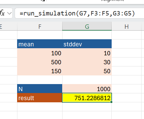
@xl_func("int n, float[] means, float[] stddevs: float")
def run_simulation(n, means, stddevs):
results = []
for _ in range(n):
# draw some random samples
cost_estimates = np.random.normal(means, stddevs)
# our "model" is just the sum of the estimates
results.append(cost_estimates.sum())
# return the mean of all the results
return sum(results) / n
The function takes a number of times to run the model (n), a list of the mean for the cost estimates (means) and a list of the standard deviations of the cost estimates (stddevs).
The @xl_func decorator tells the PyXLL add-in to make this function available to us in Excel. We have given it a “signature string” to tell it the types of the arguments, and the return type. PyXLL uses this when it exposes the function to Excel, so it can be called correctly.
Step 2: Running the simulation in Excel
To run your Python code in Excel you need to first have the PyXLL add-in installed. You can find instructions for how to do that here https://www.pyxll.com/docs/userguide/installation/index.html.
Once you have PyXLL installed and working, you just need to add your Python module to the “modules” list in the pyxll.cfg configuration file. You should also add the folder you’ve saved the module to the “pythonpath” setting in the same file, if it’s not included there already.
After doing that, start Excel (or click “Reload” in the PyXLL menu to reload the Python code) and the “run_simulation” function we wrote above is now available to be called directly from the worksheet!
Step 3: Getting the standard deviation of our result
In steps 1 and 2 we saw how we can write a Python function and call it from Excel, but currently that function only returns us the mean result. To understand how certain that result is we need to also calculate the standard deviation of the result.
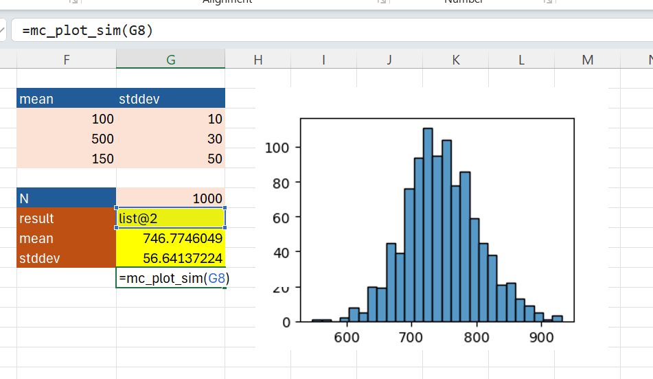
Instead of returning just a number, we can return the entire list of results. But, we don’t want to see those as a massive list in Excel! We might be doing many thousands of samples and there’s no need for us to see every single one and it would take up too much space in our workbook.
So, we change the return type in the @xl_func decorator to “object”. This returns the Python object to Excel as a single value object reference. We can then pass that to other Python functions. We’ll write two more functions as well, one to calculate the mean and one to calculate the standard deviation:
from pyxll import xl_func, xl_app
import numpy as np

@xl_func("int n, float[] means, float[] stddevs: object")
def run_simulation(n, means, stddevs):
    results = []
    for _ in range(n):
        # draw some random samples
        cost_estimates = np.random.normal(means, stddevs)

        # our "model" is just the sum of the estimates
        results.append(cost_estimates.sum())

    # return all the results
    return results

@xl_func("object results: float")
def mc_mean(results):
    """Return the mean of a list of results."""
    if not results:
        return "# No results"
    return np.mean(results)


@xl_func("object results: float")
def mc_stddev(results):
    """Return the standard deviation of a list of results."""
    if not results:
        return "# No results"
    return np.std(results)
When the “run_simulation” function runs in Excel we get an object handle returned, which we then pass to our new functions “mc_mean” and “mc_stddev”.

Step 4: Plotting the results as a histogram
Getting the mean and standard deviation is useful, but sometimes it helps to see the data plotted as a histogram. With PyXLL we can use all of the major Python plotting libraries. Seaborn is one of those plotting libraries, and that’s what we’ll use to plot the histogram of results.
We’ll write one more Python function. This one takes the list of results, as the “mc_mean” and “mc_stddev” functions do, but rather than returning a number, this function will plot a chart using the PyXLL “plot” function:
import matplotlib.pyplot as plt
import seaborn as sns

@xl_func("object results: str")
def mc_plot_sim(results):
    """Plot the results of a simulation run."""
    # create a matplotlib figure and axes to plot to
    fig, ax = plt.subplots()

    # use Seaborn to plot the results as a histogram
    sns.histplot(results, ax=ax)

    # Display the figure in Excel
    plot(fig)
This is a (very) simple example. In the next section we’ll get in to how to do apply the same basic technique but where the model itself is built in Excel.
Monte Carlo for Excel Models
In the sections above we saw how we can write Python functions and call from them from Excel. We wrote a simple function that ran a simple model to generate total cost estimates drawing from a set of normal distributions.
Real world cases are more complex than this and very often we want to build the model part in Excel. For example, if you have a spreadsheet that calculates total cost (or it could be anything) from some input assumptions, you might want to know what the output would look like if those input assumptions were drawn from distributions rather than being fixed numbers.
You might have done something where you know roughly what your input numbers are and put those in Excel, but then you think “what if this number increases by 10%”, or something like that, and so you do some experiments seeing how different inputs affect the output to get a feel for the model. Monte Carlo is like that, but with a little more mathematical rigor behind it.
What we’ll do in this next section is see how we can use PyXLL and Python to vary inputs to an Excel model, using a Monte Carlo style approach, sample the output value as calculated by Excel, and present the results.
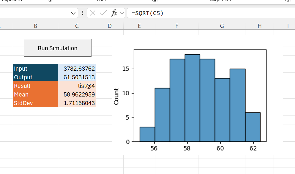
Tweaking Excel Model Inputs
The basic idea of what we’re building is that we will have a model in Excel with the output in one cell, and some inputs in some other cells. We will control the inputs using defined distributions. We change the inputs using samples from those distributions and observe the output.
For this we’ll use an Excel macro (often called “Sub” in VBA circle) instead of a worksheet function. The following code sets the value in one cell and samples the output calculated in another.
For a guide to writing Excel macros in Python, see https://www.pyxll.com/docs/userguide/macros.html
from pyxll import xl_macro, XLCell
from pert import PERT  # requires "pertdist"
import numpy as np

@xl_macro
def run_simulation():
    # Create an example distribution and draw some samples from it
    dist = PERT(3000, 3500, 4000)
    samples = dist.rvs(100)

    # Get the (single) input and output cells, hardcoded for now
    input = XLCell.from_range("C5")
    output = XLCell.from_range("C6")

    results = []
    for x in samples:
        # Update the input cell value
        input.value = x

        # Collect the output cell value
        results.append(output.value)

    # Write the results to another cell
    result_cell = XLCell.from_range("C7")
    result_cell.options(type="object").value = results
We assign this macro to a button in Excel, and when we press the button, the code runs, updates the input cell, and collects the results.
The macro writes results to cell C7, and we can then pass those results to our “mc_mean", “mc_stddev", and “mc_plot_sim" functions just as we did in the section above.
Defining the Random Variables in Excel
The above example has several limitations, especially because the code hard-codes the random distribution used for the input. Instead we would like to be able to decide what distribution to use for each variable from Excel.
To do this we will write some new Python functions that return “RandomVariable” objects, which can then be used in our simulation. We’ll write a new RandomVariable class with methods get samples from the random distribution, and we’ll also give them the ability to update an Excel cell with a sampled value.
As we might want to use various different types of distribution, we’ll make RandomVariable an abstract base class. Later, we can write implementations of this class for any type of distribution we want.
from abc import ABCMeta, abstractmethod

class RandomVariable(metaclass=ABCMeta):
    """Base class for random variables."""

    # Each random variable has a name (which will be useful later for plotting)
    # and also a target cell. The target cell is the input to the Excel model that
    # we overwrite with simulated values.
    def __init__(self, name: str, target: XLCell):
        self.name = name
        self.target = target

    @abstractmethod
    def samples(self, n, seed=None):
        """Return n random samples."""
        pass

    def simulate(self, value):
        self.target.value = value
Above we used the PERT distribution, and we can implement a new class derived from the RandomVariable base class that implements samples using that same distribution:
class PertRandomVariable(RandomVariable):
    """Random variable using the PERT distribution."""

    def __init__(self,
                 name: str,
                 target: XLCell,
                 min_value: float,
                 ml_value: float,
                 max_vaue: float,
                 lamb: float = 4.0):
        super().__init__(name, target)
        self.__dist = PERT(min_value, ml_value, max_vaue, lamb)

    def samples(self, n, seed=None):
        return self.__dist.rvs(size=n, random_state=seed)
Finally we need a way to create this “PertRandomVariable” object in Excel, which we do via an Excel function using the @xl_func decorator:
@xl_func("string, xl_cell, float, float, float, float: object")
def mc_pert(name, target, min_value, ml_value, max_vaue, lamb=4.0):
    """Returns a RandomVariable object instance using the PERT distribution."""
    return PertRandomVariable(name, target, min_value, ml_value, max_vaue, lamb)
Note the type of the “target” argument is “xl_cell”. This tells the PyXLL add-in to pass a cell reference object to the function instead of the cell value.
We can add the call to the new “mc_pert” to our sheet, using “C5” as the target input cell.
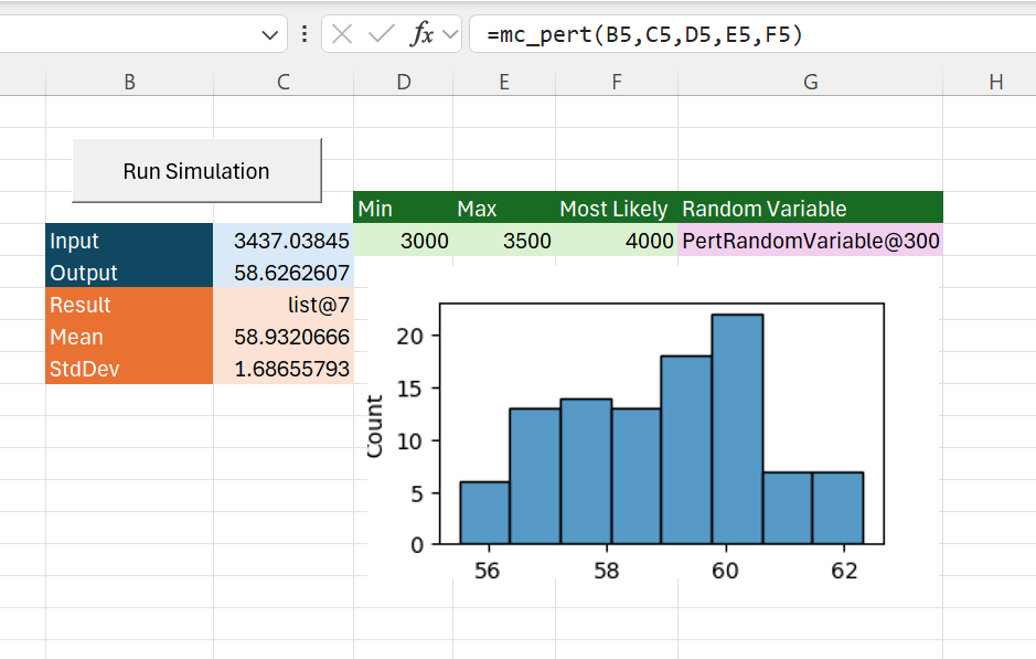
Our macro needs updating to get the random variable from cell G5, and to use that to get the random samples and set the target cell value:
@xl_macro
def run_simulation():
    # Get the random input variable as a Python object
    rv_cell = XLCell.from_range("G5")
    rv = rv_cell.options(type="object").value

    # and output cell
    output = XLCell.from_range("C6")

    results = []
    for x in rv.samples(100):
        # Update the input cell value
        rv.simulate(x)

        # Collect the output cell value
        results.append(output.value)

    # Write the results to another cell
    result_cell = XLCell.from_range("C7")
    result_cell.options(type="object").value = results
We now have a working Monte Carlo solution in Excel! We can use any Excel formula as the output, and we can customize the parameters of the input distribution.
Although it still has limitations, it provides a good start. The remaining issues we need to resolve are
- We want to have multiple inputs to our model, not just one
- There is no way to enter the number of samples currently
- It is quite slow to run the simulation
- The final macro should not have cell references hard-coded into it
The next sections address these issues.
Multiple Input Variables
The current “run_simulation” macro takes a single random variable input from a cell reference. Instead, we would like to be able to have multiple inputs to our model controlled by different distributions, without having to update the macro to list all of those inputs.
A good way to deal with these various inputs is to collect them all into a single “Simulation” object. We’ll create a new class for that to hold all of the input random variables, the output cell, and the number of samples we want to run the simulation over.
class Simulation:
    """Simulation class for managing setting inputs to random variables
    and collecting the calculated output.
    """

    def __init__(self,
                 name: str,
                 n: int,
                 output: XLCell,
                 inputs: list[RandomVariable]):
        self.name = name
        self.n = n
        self.output = output
        self.inputs = inputs

    def run(self):
        results = []

        # Prepare random samples for the inputs
        samples = [input.samples(self.n, seed=seed) for input in self.inputs]

        # Calculate the output value for each set of inputs
        for i in range(self.n):
            # Get the sample value for each input and set it
            for j, input in enumerate(self.inputs):
                input_samples = samples[j]
                value = input_samples[i]
                input.simulate(value)

            # Collect the output value with the input values set
            results.append(self.output.value)

        return results
As previously, we also now need an Excel function to create this new Simulation object:
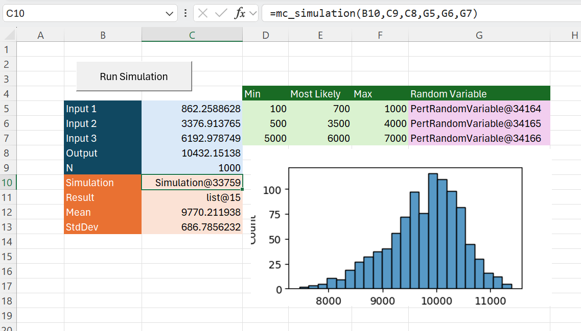
@xl_func("str name, int n, xl_cell output, object *inputs: object")
def mc_simulation(name, n, output, *inputs):
    """Returns a Simulation object for use with the 'mc_run_simulation' macro."""
    return Simulation(name, n, output, inputs)
This “mc_simulation” function takes any number of input variables. Now we update the spreadsheet to add some more variables and add our simulation object:
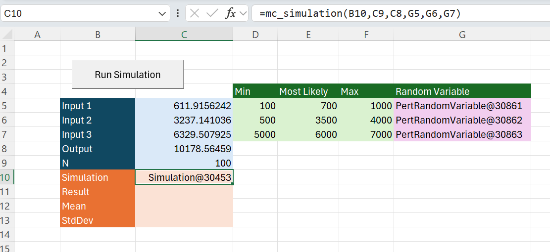
The “run_simulation” macro needs an update to use the simulation object in cell C10.
@xl_macro
def run_simulation():
    # Get the simulation object from cell C10
    cell = XLCell.from_range("C10")
    simulation = cell.options(type="object").value

    # Run the simulation
    results = simulation.run()

    # And write the results to cell below
    cell.offset(rows=1).options(type="object").value = results
Our “run_simulation” macro is much simpler than before and now only has the cell C10 hard-coded in it (and we will fix that soon…).
Run Faster
You might have noticed that updating the input cells and recalculating the output takes a little while.
Part of the problem is that whenever any of our input cells change, Excel recalculates the output cell. Now that we’re updating multiple input cells, Excel does too much work – we only need the output after all input cells are updated.
The other thing that slows things down is Excel is re-drawing the screen every time there is an update. This takes more time than you might expect and causes the whole calculation to be much slower than it needs to be.
PyXLL has a convenient solution for this! The context manager pyxll.xl_disable() switch Excel to manual calculation mode and disables screen updating! Because calculations will be set to manual when using this, we now need to calculate the output cell manually.
from pyxll import xl_disable

class Simulation:
    """Simulation class for managing setting inputs to random variables
    and collecting the calculated output.
    """

    def __init__(self,
                 name: str,
                 n: int,
                 output: XLCell,
                 inputs: list[RandomVariable]):
        self.name = name
        self.n = n
        self.output = output
        self.inputs = inputs

    def run(self):
        results = []

        # Prepare random samples for the inputs
        samples = [input.samples(self.n) for input in self.inputs]

        output_range = self.output.to_range()

        # Disable automatic calculations and screen updating
        with xl_disable():
            for i in range(self.n):
                # Get the sample value for each input and set it
                for j, input in enumerate(self.inputs):
                    input_samples = samples[j]
                    value = input_samples[i]
                    input.simulate(value)

                # Calculate the output range
                output_range.Calculate()

                # Collect the output value
                results.append(self.output.value)

        return results
And with that small change our simulation now runs much much faster!
Removing the last hard coded cell
We still have cell C10 hardcoded in our macro. This is not ideal as we might want to use the same macro to run different Monte Carlo simulations, and we don’t want to rely on the simulation object always being in cell C10!
We can’t pass arguments or parameters directly to a macro function from a button, but what we can do it get the button from inside the macro. We can add some data to the button and then read it back in the macro. One convenient place to add data like this is in the button’s Alternative Text field.
Right click the button, go to Format Control, and find the “Alt Text” tab. That’s where we’ll store the cell reference for the simulation object.
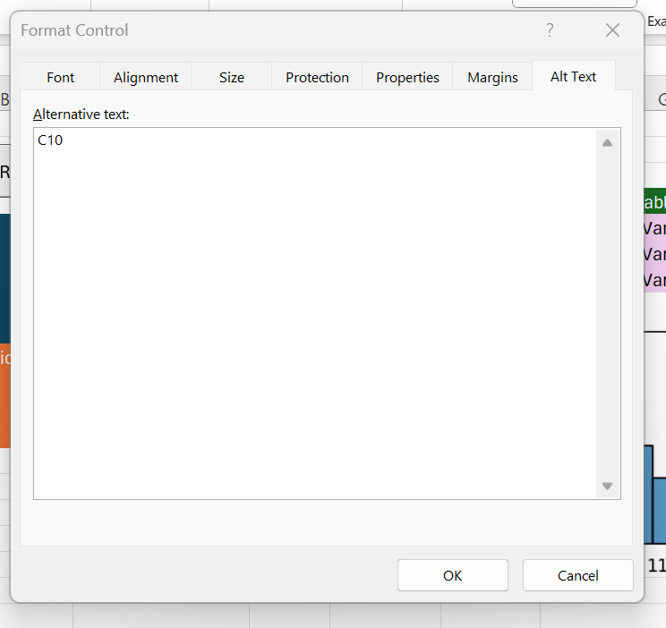
The only remaining thing to do now is to fetch that in our macro as follows:
@xl_macro
def mc_run_simulation():
    """Run a Simulation located at the cell specified in the calling button's
    alternative text field.
    """
    # Get the cell reference from the calling button's Alternative Text
    xl = xl_app()
    caller = xl.Caller
    button = xl.ActiveSheet.Shapes[caller]
    address = button.AlternativeText

    # Get the simulation object from the cell address
    cell = XLCell.from_range(address)
    simulation = cell.options(type="object").value

    # Run the simulation
    results = simulation.run()

    # And write the results to cell below
    cell.offset(rows=1).options(type="object").value = results
Further Improvements
There are various things you could do to continue to improve on this, but hoepefully the above will get you off to a good start!
You can find a version of this code, along with some more improvements, on GitHub here https://github.com/pyxll/pyxll-examples/blob/master/montecarlo
Some of the improvements in the code linked above include
- Progress indicator
- Better error reporting
- Resetting the inputs after the simulation
- Plotting the input distributions
See the video https://youtu.be/Va9ih1DXPDs for a walkthrough of all of this code in detail.