
- Introduction
- Write code to run inside and outside of Excel
- Setting up the Example
- How long is it taking?
- How to speed up your Python code
- Resources
Introduction
All the code from this blog is on github
When creating any kind of application, there sometimes comes a point where things are not running as smoothly as you want and you need to think about the performance of your application. The same is true when developing Excel spreadsheets. Using PyXLL to add functionality to Excel is an extremely powerful way to create rich analytics and applications in Excel, but what do you do when your Python based spreadsheet is having performance problems?
When tackling any sort of performance problem, the first step is always to profile the code! This post covers some pointers to make it easier for you to identify performance bottlenecks (or hotspots) and how to profile a running Excel application.
Write code to run inside and outside of Excel
When writing Python code for Excel it’s helpful to be able to run it outside of Excel as well. Doing so means that you can apply automated testing (e.g. unit testing) to your code, and also you can examine any performance bottlenecks and debug problems without having to run your code in Excel.
To help you do this, PyXLL provides as stubs package that declares all the same functions and decorators you use to expose your Python functions to Excel (e.g. @xl_func), but that do nothing. This means you can run the same code both in Excel and from any Python prompt.
When you download PyXLL, the stubs package is provided as a .whl file, or Python Wheel. It will be named pyxll-{version}-{pyversion}-none-win{32/64}.whl, depending on which version of Python you have downloaded PyXLL for. To install it, open a command prompt and if necessary active your Python environment and use the command pip to install the whl file:
>> activate myenv  ;; only if using conda or a venv
>> pip install ./pyxll-3.5.4-cp36-none-win_amd64.whl [/code]
Note:Use the path to the file, including “./” if in the current directory. Without this, pip will look for a wheel with that name from the remote PyPI repository instead of installing the local file.
Now you will be able to import pyxll from Python even if not running in Excel via the PyXLL add-in.
Setting up the Example
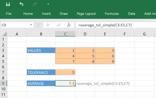
Before we can look at profiling, we need to set up some code to profile 🙂 For this we’ll use a simple function that calculates the average of a range of numbers, with a tolerance so only numbers above that tolerance are included.
An example function
Start your preferred Python IDE (I will be using PyCharm for this blog), or a simple text editor will do, create a new file named “average_tol.py” and enter the following:
from pyxll import xl_func

@xl_func
def average_tol_simple(values, tolerance):
    """Compute the mean of values where value is > tolerance

    :param values: Range of values to compute average over
    :param tolerance: Only values greater than tolerance will be considered
    """
    total = 0.0
    count = 0
    for row in values:
        for value in row:
            if not isinstance(value, float):
                continue
            if value <= tolerance:
                continue
            total += value
            count += 1
    return total / count
This function will compute the average of a range of numbers above the specified tolerance, and will also be available to be called from Excel because it’s decorated with the @xl_func annotation.
We can test this by importing the Python module and calling the function. If you are using PyCharm you can right click and select “Run File in Console”. This will run the file and give you an IPython prompt so you can test the function:
In[2]: average_tol_simple([[1,2,3],[4,5,6],[7,8,9]], 5)
Out[2]: 7.5
If you are not using PyCharm, you can import the function and run it as normal from an IPython prompt. If you don’t have IPython installed, install it now as we will be using some of its timing features later. IPython can be installed by running “pip install ipython” or “conda install ipython” if you are using Anaconda.
Setting up Excel
Now we’ve got a basic function we can try calling it from Excel. If you’ve not already installed PyXLL, install it now. See the PyXLL Introduction for installation instructions. Ensure you point it at the same Python you have been using so far by setting “executable” in the pyxll.cfg config file.
Once you’ve got PyXLL installed successfully, add the path where you’ve saved “average_tol.py” to your Python path and add “average_tol” to the list of modules for PyXLL to import:
[PYTHON]
executable = {path to your Python executable}
pythonpath =
    {path to the folder where average_tol.py is saved}

[PYXLL]
modules =
    average_tol
Now when you reload PyXLL (or restart Excel) our new “average_tol_simple” function will be available to call as a worksheet function.
How long is it taking?
Measuring how long a function takes
Now we’ve got a basic function working in Excel, how long does it take to run? If it’s very slow, we can just time it roughly using a watch or the clock on the computer. That’s error prone and won’t really give us the precision we need. Luckily, IPython has a way to time how long it takes to run a function accurately. It does this by running the function a number of times and taking the average.
To time the function in IPython we use the “%timeit” command. To make the function take a little longer, we’ll use a range with 32,000 values. To get that range, we use numpy’s arange function and reshape it into a 2d array.
[In2]: values = np.arange(1, 32001, dtype=float).reshape((320, 100))
[In3]: average_tol_simple(values, 500)
Out[2]: 16250.5
[In4]: %timeit average_tol_simple(values, 500)
14.9 ms ± 135 µs per loop (mean ± std. dev. of 7 runs, 100 loops each)
Great! So on my laptop, it takes about 15ms to run that function for 32,000 values. But, how long does the same function take in Excel? We’d expect it to be a slower since there is inevitably some overhead in constructing the Python array from the Excel values and calling the Python function, but how can we test that?
One way is to set up the calculation we want, and then add a menu function to trigger that calculation and time how long Excel takes to do it. There will be some cost involved in calling the Excel API to run the calculation, but if we run a long enough calculation that time will be insignificant and so we can get a reasonably accurate picture of how long it’s taking.
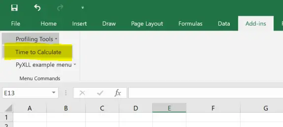
The following triggers the recalculation of the selected cell 100 times and calculates the mean time and standard deviation. This is roughly the same as what we did previously using “%timeit” in IPython. To use it, copy the following code to a new file called “profiling_tools.py” and add “profiling_tools” to the list of modules in your pyxll.cfg file. When you reload PyXLL you will see a new menu “Profiling Tools” (under the Add-Ins tab) with our new menu item “Time to Calculate.
from pyxll import xl_menu, xl_app, xlcAlert
from win32com.client import constants
import win32clipboard
import math
import time

@xl_menu("Time to Calculate", menu="Profiling Tools")
def time_calculation():
    """Recalculates the selected range and times how long it takes"""
    xl = xl_app()

    # switch Excel to manual calculation and disable screen updating
    orig_calc_mode = xl.Calculation
    try:
        xl.Calculation = constants.xlManual
        xl.ScreenUpdating = False

        # get the current selection
        selection = xl.Selection

        # run the calculation a few times
        timings = []
        for i in range(100):
            # Start the timer and calculate the range
            start_time = time.clock()
            selection.Calculate()
            end_time = time.clock()
            duration = end_time - start_time
            timings.append(duration)
    finally:
        # restore the original calculation mode and enable screen updating
        xl.ScreenUpdating = True
        xl.Calculation = orig_calc_mode

    # calculate the mean and stddev
    mean = math.fsum(timings) / len(timings)
    stddev = (math.fsum([(x - mean) ** 2 for x in timings]) / len(timings)) ** 0.5
    best = min(timings)
    worst = max(timings)

    # copy the results to the clipboard
    data = [
        ["mean", mean],
        ["stddev", stddev],
        ["best", best],
        ["worst", worst]
    ]
    text = "\n".join(["\t".join(map(str, x)) for x in data])
    win32clipboard.OpenClipboard()
    win32clipboard.EmptyClipboard()
    win32clipboard.SetClipboardText(text)
    win32clipboard.CloseClipboard()

    # report the results
    xlcAlert(("%0.2f ms \xb1 %d \xb5s\n"
              "Best: %0.2f ms\n"
              "Worst: %0.2f ms\n"
              "(Copied to clipboard)") % (mean * 1000, stddev * 1000000, best * 1000, worst * 1000))
Note:If you can’t import win32clipboard you need to install the pywin32 package. You can do that with pip, “pip install pypiwin32” or with conda, “conda install pywin32”.
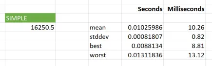
In Excel we can now use this menu item to time how long an individual cell (or range of cells) takes to calculate. Modifying the call to “average_tol_simple” to take a range with 32,000 values and using this, on my PC I get a result that it takes about 11 ms to compute. This is actually lower than it took in IPython! However, that’s because in IPython we were iterating over a numpy array which is slower than iterating over the list that we get with PyXLL. For a fair comparison we need to use a list in both cases and then we see that the time take in IPython is lower:
[In5]: values2 = values.tolist()
[In6]: %timeit average_tol_simple(values2, 500)
8.14 ms ± 37.2 µs per loop (mean ± std. dev. of 7 runs, 100 loops each)
Now the time in Excel is slightly longer than in IPython, as expected due to passing 32,000 values between Excel and Python.
Profiling an Excel Application
Sometimes when a workbook is running slowly it’s not obvious where that time is being spent. It’s easy to speculate and guess what function is taking a long time, but to be sure it’s always good practice to profile. Even if you think you know where the problem is, you can often be surprised after profiling!
Python comes with its own profiler called cProfile.
To profile a Python script, cProfile can be run as follows:
python -m cProfile -s cumtime your_script.py
This prints out all the functions called, with the time spend in each and the number of times they have been called.
As mentioned earlier, if you can run your code outside of Excel and can build a script that runs your functions with representative data then that makes things nice and easy 🙂 You can just run that script using cProfile and see where the bottlenecks are!
Real world cases are rarely that straightforward, and in order to get to the point where we can focus on a few functions outside of Excel we need to profile what Excel is actually doing. Starting to optimize your code without profiling first will waste a lot of time.
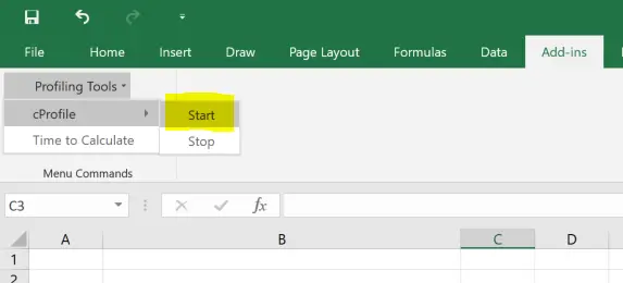
We can call the cProfile module from inside Excel from a couple of menu functions. By starting and stopping the profiler in Excel we can get some details about what’s actually being called. The following code adds two new menu items, one for starting the profiler and another for stopping it and collecting the results.
from pyxll import xl_menu, xlcAlert
from io import StringIO
import win32clipboard
import cProfile
import pstats

_active_cprofiler = None

@xl_menu("Start", menu="Profiling Tools", sub_menu="cProfile")
def start_profiling():
    """Start the cProfile profiler"""
    global _active_cprofiler
    if _active_cprofiler is not None:
        _active_cprofiler.disable()
    _active_cprofiler = cProfile.Profile()

    xlcAlert("cProfiler Active\n"
             "Recalcuate the workbook and then stop the profiler\n"
             "to see the results.")

    _active_cprofiler.enable()

@xl_menu("Stop", menu="Profiling Tools", sub_menu="cProfile")
def stop_profiling():
    """Stop the cProfile profiler and print the results"""
    global _active_cprofiler
    if not _active_cprofiler:
        xlcAlert("No active profiler")
        return

    _active_cprofiler.disable()

    # print the profiler stats
    stream = StringIO()
    stats = pstats.Stats(_active_cprofiler, stream=stream).sort_stats("cumulative")
    stats.print_stats()

    # print the results to the log
    print(stream.getvalue())

    # and copy to the clipboard
    win32clipboard.OpenClipboard()
    win32clipboard.EmptyClipboard()
    win32clipboard.SetClipboardText(stream.getvalue())
    win32clipboard.CloseClipboard()

    _active_cprofiler = None

    xlcAlert("cProfiler Stopped\n"
             "Results have been written to the log and clipboard.")
Copy the code above into “profiling_tools.py” and add “profiling_tools” to the list of modules in your pyxll.cfg. Restart PyXLL and you’ll find the new menu items should have been added to the Add-Ins menu.
To profile your workbook, start the profiler using the menu item and then recalculate everything you want to be included in the profile. When finished, stop the profiler and the results are printed to the log file and copied to the clipboard.
         32024 function calls (32023 primitive calls) in 0.020 seconds

   Ordered by: cumulative time

   ncalls  tottime  percall  cumtime  percall filename:lineno(function)
        1    0.009    0.009    0.012    0.012 c:\github\pyxll-examples\profiling\average_tol.py:8(average_tol_simple)
      2/1    0.005    0.002    0.005    0.005 c:\github\pyxll-examples\profiling\average_tol.py:49(average_tol_numba)
        1    0.003    0.003    0.003    0.003 c:\github\pyxll-examples\profiling\average_tol.py:28(average_tol_try_except)
    32002    0.003    0.000    0.003    0.000 {built-in method builtins.isinstance}
Once you’ve identified what functions are taking most time you can focus on improving them.
Profiling multi-threaded Python code
The Python profiler cProfile used in the section above is great for single threaded code, but it only collects profiling data for the thread it’s called on. It is common to use one or more background threads when writing RTD or async functions, and using cProfile in these cases will not include timing data for the background threads.
Fortunately there is another third-party profiling tool, yappi that will profile code running in all threads. Yappi can be installed using pip:
>> pip install yappi
Profiling using yappi is straightforward and can be done in a similar way to what was shown above. All that is needed is to modify the start_profiling and stop_profiling menu functions to use yappi instead of cPython.
@xl_menu("Start", menu="Profiling Tools", sub_menu="Yappi")
def start_profiling():
    yappi.start()

@xl_menu("Stop", menu="Profiling Tools", sub_menu="Yappi")
def stop_profiling():
    yapp.stop()
    yappi.get_func_stats().print_all()
    yappi.get_thread_stats().print_all()
    yappi.clear_stats()
The procedure to profiling your code is the same as above. Start the profiler, recalculate everything you want to profile and then stop the profiler. The results will be written to the log file, only this time everything from any background threads will also be included.
How to speed up your Python code
Optimizing Python code is a whole series of blog posts in itself, but since now we know how to time an individual function in both IPython and Excel it’s a good time to dig a little deeper and see how we can improve things.
Line Profiling
If you already know what function you need to spend time optimizing then the “line_profiler” Python package is a useful tool to drill into the function and see where the time’s going. In our case, since we only have one function we know which one to optimize, but in more complex cases it’s advisable to spend some time before this stage to uncover exactly which functions are problematic.
Install the “line_profiler” package using “pip install line_profiler” or “conda install line_profiler” if using Anaconda.
The line profiler works by running a Python script and looking for functions decorated with a special ‘@profile’ decorator. The easiest way to run it for our function is to turn the module into script that will call the function we’re interested in a number of times. We do this by adding some code at the end that only runs if the module is being run as a script by checking __name__ == “__main__”.
from pyxll import xl_func

@xl_func
@profile
def average_tol_simple(values, tolerance):
    """Compute the mean of values where value is > tolerance

    :param values: Range of values to compute average over
    :param tolerance: Only values greater than tolerance will be considered
    """
    total = 0.0
    count = 0
    for row in values:
        for value in row:
            if not isinstance(value, (float, int)):
                continue
            if value <= tolerance:
                continue
            total += value
            count += 1
    return total / count

if __name__ == "__main__":
    import numpy as np
    values = np.arange(1, 32001, dtype=float).reshape(100, 320).tolist()
    for i in range(100):
        avg = average_tol_simple(values, 500)
Note that now “@profile” has been added to the average_tol_simple function.
To run the line profiler we do the following:
>> kernprof -v -l average_tol.py
The “-v” option tells the profiler to print the results rather than save them to a file. On my PC, the results look like this:
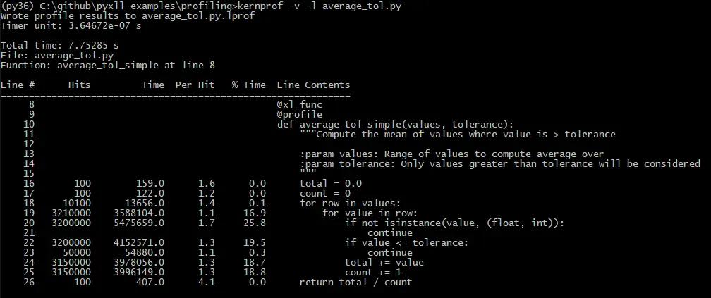
Looking at the percentage time we can see that the biggest contributor is testing whether the value is a number of not. In Python, using a try/except block can be faster than doing explicit checks like this so we can try removing that check and catching and TypeError exceptions that might be raised as follows:
def average_tol_try_except(values, tolerance):
    total = 0.0
    count = 0
    for row in values:
        for value in row:
            try:
                if value <= tolerance:
                    continue
                total += value
                count += 1
            except TypeError:
                continue
    return total / count
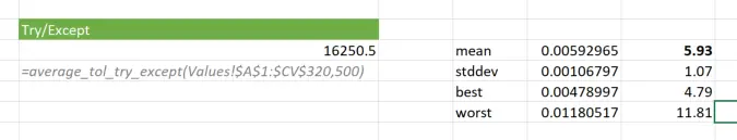
Using IPython’s %timeit again we can see that change has really improved the performance of this function.
[In8]: %timeit average_tol_try_except(values, 500)
3.53 ms ± 60.8 µs per loop (mean ± std. dev. of 7 runs, 100 loops each)
Running the same test as before in Excel also shows a similar speed up, though because we are passing a large range of data and the function the time taken to convert the data from Excel to Python means there is always some small overhead.
Using the Line Profiler in Excel
As well as using the line profiler from the command line as described above, it’s also possible to use the line_profiler API to profile functions without leaving Excel.
The following code adds two new menu items to start and stop the line profiler. Once the line profiler is started, if any function decorated with the @enable_line_profiler decorator (also defined below) will be profiled. When the profiler is stopped the results are written to the log file and to the clipboard to be pasted into Excel.
from pyxll import xl_menu
from functools import wraps
from io import StringIO
import win32clipboard
import line_profiler

# Current active line profiler
_active_line_profiler = None

@xl_menu("Start", menu="Profiling Tools", sub_menu="Line Profiler")
def start_line_profiler():
    """Start the line profiler"""
    global _active_line_profiler
    _active_line_profiler = line_profiler.LineProfiler()

    xlcAlert("Line Profiler Active\n"
             "Run the function you are interested in and then stop the profiler.\n"
             "Ensure you have decoratored the function with @enable_line_profiler.")

@xl_menu("Stop", menu="Profiling Tools", sub_menu="Line Profiler")
def stop_line_profiler():
    """Stops the line profiler and prints the results"""
    global _active_line_profiler
    if not _active_line_profiler:
        return

    stream = StringIO()
    _active_line_profiler.print_stats(stream=stream)
    _active_line_profiler = None

    # print the results to the log
    print(stream.getvalue())

    # and copy to the clipboard
    win32clipboard.OpenClipboard()
    win32clipboard.EmptyClipboard()
    win32clipboard.SetClipboardText(stream.getvalue())
    win32clipboard.CloseClipboard()

    xlcAlert("Line Profiler Stopped\n"
             "Results have been written to the log and clipboard.")

def enable_line_profiler(func):
    """Decorator to switch on line profiling for a function.

    If using line_profiler from the command line, use the built-in @profile
    decorator instead of this one.
    """
    @wraps(func)
    def wrapper(*args, **kwargs):
        nonlocal func
        if _active_line_profiler:
            func = _active_line_profiler(func)
        return func(*args, **kwargs)
    return wrapper
Copy the code above into your profiling_tools.py file, and add the @enable_line_profiler decorator to the average_tol_simple function.
from pyxll import xl_func
from profiling_tools import enable_line_profiler

@xl_func
@enable_line_profiler
def average_tol_simple(values, tolerance):
    total = 0.0
    count = 0
    for row in values:
        for value in row:
            if not isinstance(value, (float, int)):
                continue
            if value <= tolerance:
                continue
            total += value
            count += 1
    return total / count
Now reload PyXLL and you’ll see the two new menu items. Start the line profiler, call average_tol_simple, then stop the line profiler and copy the results to Excel or look at the log file.
Use NumPy or Pandas to replace for loops
For operations involving large arrays of data it’s often much faster (and simpler) to use numpy or pandas rather than writing for loops to process data.
Our example function can easily be re-written using numpy:
@xl_func("numpy_array<float>, float: float")
def average_tol_numpy(values, tolerance):
    return values[values > tolerance].mean()
Note the use of the signature in @xl_func. That tells PyXLL what types to pass to our function, and so handles the conversion of the array of data into a numpy array for us.
This function is significantly faster than our original, and now the time taken is dominated by the cost of converting the Excel data into Python objects.
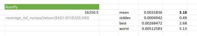
[In9]: %timeit average_tol_numpy(values, 500.0)
61.5 µs ± 451 ns per loop (mean ± std. dev. of 7 runs, 10000 loops each)
This version of the function however doesn’t handle non-numeric types being passed to it, whereas the previous ones would skip non-numeric values. Adding those checks back in negates the improvement gained by using numpy, which goes to show why profiling is so important!
Speed up your code using Numba or Cython
For certain types of CPU bound functions you can get significant speedups using Numba or Cython.
Numba is a Python JIT compiler that can speed up any array and math heavy calculations with simple annotations. For example, all that’s need to speed up our average function is to do the following:
from pyxll import xl_func
import numba

@xl_func
@numba.jit(locals={"value": numba.double, "total": numba.double, "count": numba.int32})
def average_tol_numba(values, tolerance):
    total = 0.0
    count = 0
    for row in values:
        for value in row:
            if value <= tolerance:
                continue
            total += value
            count += 1
    return total / count
By telling Numba some of the types of the local variables it can the code faster. However, for a function like this where most of the time is spent iterating over the lists, the overhead of using the JIT compiler means there is little or no performance benefit. Real world functions are likely to have better results!
Cython works by converting Python code into C code, which is then compiled into a C extension. When used carefully this can speed up code dramatically. As with all optimization techniques though, constant profiling is required to understand where the time is being spent.
Multi-threading
Excel can run calculations concurrently across multiple threads. This is only applicable if the functions can actually be run concurrently and don’t depend on each other. For sheets with many functions this can improve the overall time to calculate the sheet by making better use of a modern PCs’ multiple cores.
To enable a function to be run in a background calculation thread, all that’s required is to add “thread_safe=True” to the “@xl_func” decorator:
from pyxll import xl_func

@xl_func(thread_safe=True)
def thread_safe_func():
    pass
Although thread safe functions may be run concurrently across multiple threads, Python code can’t always take advantage of this because of something called the “GIL” or “Global Interpreter Lock”. Basically, while the Python interpreter is doing anything it always acquires the GIL, preventing any other thread from running any Python code at the same time! This means that although your Python code is now running on multiple threads, it only runs on one thread at once and so you see no benefit from this.
All is not lost however. Many libraries will release the GIL while running long tasks. For example, if you are reading a large file from disk, then Python will release the GIL while that IO operation takes place meaning that it’s freed up for other threads to continue running Python code. Packages like numpy and scipy also release the GIL while performing numerical computations, so if you are making heavy use of those your code may benefit from being multi-threaded too. If you are using numba or cython to speed up your code, both of those have options to release the GIL so you can make your code thread friendly.
If you have IO bound functions (e.g. reading from disk, a network or a database), or if you’re packages that release the GIL (like numpy or scipy), then using multiple threads may help. If your functions are purely CPU bound and are just running plain Python code then it may not.
For some more information about multi-threading and multi-processing in Python see this post: https://www.geeksforgeeks.org/difference-between-multithreading-vs-multiprocessing-in-python/.
For a more detailed explanation of the GIL see https://wiki.python.org/moin/GlobalInterpreterLock.
Asynchronous Functions
For IO bound functions asynchronous functions allow Excel to continue working on other functions while the asynchronous function continues in the background. This can be useful in some situations where you don’t want to block one of the calculation threads from doing other calculations while you wait for a response from a remote server, for example.
For more information about asynchronous functions in PyXLL see Asynchronous Functions in the user guide.
Note that asynchronous functions must still return during Excel’s calculation phase, and so they are not a way to free up the user interface while a long running calculation is being performed. For that, use an RTD (Real Time Data) function instead.
Resources
- All the code from this blog is on github
- cProfile
- line_profiler
- Numba
- Cython
- Python Multi-Threading vs Multi-Processing
- GlobalInterpreterLock from wiki.python.org